grblc.fitting package

Submodules

grblc.fitting.constants module

grblc.fitting.io module

grblc.fitting.io.check_datatype(filename)

Given a filename, try and guess what dataset the data comes from (e.g., Si, Kann, Oates, etc.)

For example, a file named ‘*_Oates.txt’ will be interpreted as data in the same format as Sam Oates’ data.

grblc.fitting.io.check_header(path, n=None, debug=False, more_than_one_row=False)

This monstrosity returns what line a header is at

grblc.fitting.io.isfloat(value)

grblc.fitting.io.read_data(path, datatype='', debug=False)

grblc.fitting.io.readin(directory='.')

grblc.fitting.lightcurve module

class grblc.fitting.lightcurve.Lightcurve(filename: Optional[str] = None, xdata=None, ydata=None, xerr=None, yerr=None, data_space: str = 'log', name: Optional[str] = None, model: Optional[grblc.fitting.model.Model] = None, attrs: Dict[str, numpy.ndarray] = {})

Bases: object

The main module for fitting lightcurves.

Warning

Data stored in Lightcurve objects are always in logarithmic space; the parameter data_space is only used to convert data to log space if it is not already in such. If your data is in linear space [i.e., your time data is sec, and not \(log\)(sec)], then you should set data_space to lin.

Parameters

• filename (str, optional) – Name of file containing light curve data, by default None

• xdata (array_like, optional) – X values, length (n,), by default None

• ydata (array_like, optional) – Y values, by default None

• xerr (array_like, optional) – X error, by default None

• yerr (array_like, optional) – Y error, by default None

• data_space (str, {log, lin}, optional) – Whether the data inputted is in log or linear space, by default ‘log’

• name (str, optional) – Name of the GRB, by default Model name, or unknown grb if not provided.

• model (Model, optional) – Model to use in lightcurve fitting, by default None

• attrs (dict, optional) – A dict of array_like objects with length (n,) with any additional attributes (e.g., band) for each datapoint, by default {}.

fit(p0, run_mcmc=True, show=False, minimize_kwargs={}, emcee_kwargs={})

Fits the lightcurve data to the model. There are two steps in this process:

1. Minimize the residuals using Nelder-Mead with scipy.minimize

2. Probe the posterior distribution using emcee, a Markov-Chain Monte Carlo Python package, using the best-fit parameters from step 1 as the starting point. This is optional (via the run_mcmc parameter), but recommended, as it gives a better view of the errors on the best-fit parameters.

Parameters

• p0 (array_list, length of number of parameters) – Initial guess for the parameters.

• run_mcmc (bool, optional) – Whether to run the optional MCMC step, by default True

• show (bool, optional) – [description], by default False

• minimize_kwargs (dict, optional) –

  Keyword arguments to pass to scipy.minimize, by default {}

• emcee_kwargs (dict, optional) – Keyword arguments to pass to lmfit.Minimizer.emcee by default {}

Returns

See lmfit.Minimizer.MinimizerResult for more information.

Return type

lmfit.minimizer.MinimizerResult

print_fit(detailed=False)

Print a fit report to stdout.

Parameters

detailed (bool, optional) – Whether you’d like the full-on fit report, or a simplified version with the necessaries, by default False

Example:

import numpy as np
import grblc

model = grblc.Model.W07(vary_t=False)
xdata = np.linspace(0, 10, 15)
yerr = np.random.normal(0, 0.5, len(xdata))
ydata = model(xdata, 5, -12, 1.5, 0) + yerr
lc = grblc.Lightcurve(xdata=xdata, ydata=ydata, yerr=yerr, model=model)
lc.fit(p0=[4.5, -12.5, 1, 0], run_mcmc=False)
for detailed in [False, True]:
    print("="*10 + f"detailed={detailed}" + "="*10)
    lc.print_fit(detailed=detailed)

==========detailed=False==========
T	4.910507525521112	0.08532021920633912
F	-11.904896811066553	0.09041767596945684
alpha	1.4925901050996138	0.0162391180910607
t	0	0
==========detailed=True==========
[[Fit Statistics]]
    # fitting method   = Nelder-Mead
    # function evals   = 384
    # data points      = 15
    # variables        = 3
    chi-square         = 12.6502284
    reduced chi-square = 1.05418570
    Akaike info crit   = 3.44437604
    Bayesian info crit = 5.56852665
[[Variables]]
    T:      4.91050753 +/- 0.08532022 (1.74%) (init = 4.5)
    F:     -11.9048968 +/- 0.09041768 (0.76%) (init = -12.5)
    alpha:  1.49259011 +/- 0.01623912 (1.09%) (init = 1)
    t:      0 (fixed)

prompt()

A pipeline for fitting a light curve from user inputs. The data is first shown, bounds are set, parameter priors are set, and the fit is run, and saved if desired.

read_data(filename: str)

Reads in data from a file. The data must be in the correct format. See the io.read_data() for more information.

Parameters

filename (str) –

Returns

xdata, ydata, xerr, yerr

Return type

array_like

save_fit(filename=None)

Saves fit values to either a specified file or a default file.

Parameters

filename (str, optional) – File name to save fit values to, by default None

set_bounds(bounds=None, xmin=- inf, xmax=inf, ymin=- inf, ymax=inf)

Sets the bounds on the xdata and ydata to (1) plot and (2) fit with. Either

provide bounds or xmin, xmax, ymin, ymax. Assumes data is already in log space. If :py:method:`Lightcurve.set_data` has been called, then the data has already been converted to log space.

Parameters

• bounds (array_like of length 4, optional) – Bounds on inputted x and y-data, by default None

• xmin (float, optional) – Minimum x, by default -np.inf

• xmax (float, optional) – Maximum x, by default np.inf

• ymin (float, optional) – Minimum y, by default -np.inf

• ymax (float, optional) – Maximum y, by default np.inf

set_data(xdata, ydata, xerr=None, yerr=None, data_space='log')

Set the xdata and ydata, and optionally xerr and yerr of the lightcurve.

Warning

Data stored in Lightcurve objects are always in logarithmic space; the parameter data_space is only used to convert data to log space if it is not already in such. If your data is in linear space [i.e., your time data is sec, and not \(log\)(sec)], then you should set data_space to lin.

Parameters

• xdata (array_like) – X data

• ydata (array_like) – Y data

• xerr (array_like, optional) – X error, by default None

• yerr (array_like, optional) – Y error, by default None

• data_space (str, {log, lin}, optional) – Whether the data inputted is in logarithmic or linear space, by default ‘log’.

set_model(model: grblc.fitting.model.Model)

Sets the lightcurve model to use.

Parameters

model (Model) – Model to use in lightcurve fitting

show(*args, **kwargs)

Calls Lightcurve.show_fit() if a fit has been done, Lightcurve.show_data() otherwise

Returns

• *args (optional) – Positional arguments to pass to Lightcurve.show_data() or Lightcurve.show_fit()

• **kwargs (optional) – Keyword arguments to pass to Lightcurve.show_data() or Lightcurve.show_fit()

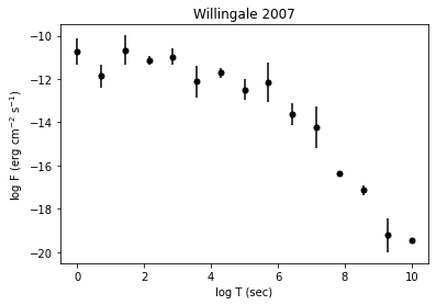
show_data(fig_kwargs={})

Plots the lightcurve data. If no fit has been ran, Lightcurve.show() will call this function.

Note

This doesn’t plot any fit results. Use Lightcurve.show_fit() to do so.

Example:

import numpy as np
import grblc

model = grblc.Model.W07(vary_t=False)
xdata = np.linspace(0, 10, 15)
yerr = np.random.normal(0, 0.5, len(xdata))
ydata = model(xdata, 5, -12, 1.5, 0) + yerr
lc = grblc.Lightcurve(xdata=xdata, ydata=ydata, yerr=yerr, model=model)
lc.show_data()

Parameters

fig_kwargs (dict, optional) – Arguments to pass to plt.figure(), by default {}.

show_fit(detailed=False, print_res=True, show_plot=True, show_corner=False, show_chisq=False, save_plots=None, show=True, corner_kwargs={}, chisq_kwargs={}, fig_kwargs={}, residual_ax_kwargs={}, fit_ax_kwargs={}, data_kwargs={}, fit_kwargs={})

Shows the fit to the data. If a fit has been ran, Lightcurve.show() will call this function.

This function can:

• Print the best-fit parameters and their errors. (print_res)

• Show the fit to the data. (show_plot)

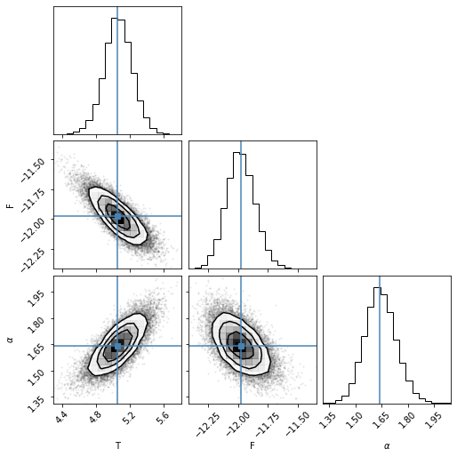
• Show the corner plot of the posterior distribution of the parameters. (show_corner)

• Show the \(\Delta\chi^2\) confidence intervals of the fit. (show_chisq)

Parameters

• detailed (bool, optional) – Whether to use all plotting and printing capabilities available to show the fit, by default False

• print_res (bool, optional) – Prints the fit result parameters and their errors, by default True

• show_plot (bool, optional) – Shows the lightcurve and fitted model, as well as residuals, by default True

• show_corner (bool, optional) – Whether to show the corner plot. Can only be used when use_mcmc was set to True when calling Lightcurve.fit(), by default False

• show_chisq (bool, optional) – Whether to show \(\Delta\chi^2\) confidence intervals, by default False

• save_plots (bool or str, optional) – If bool, whether to save the plots or not in a folder in the current directory called plots. If str, the directory and filename to save plots (e.g., ../../fit/grb010222.pdf), by default None

• show (bool, optional) – Whether you want plt.show() to be ran. If not true, the figures will be returned as a dictionary, by default True

• corner_kwargs (dict, optional) – Additional arguments to pass to corner.corner(), by default {}

• chisq_kwargs (dict, optional) – Additional arguments to pass to plt.plot for the \(\Delta\chi^2\) confidence interval plots, by default {}

• fig_kwargs (dict, optional) – Additional arguments to pass to plt.figure when showing the fit plot, by default {}

• residual_ax_kwargs (dict, optional) – Additional arguments to pass to the residual axes subplot, by default {}

• fit_ax_kwargs (dict, optional) – Additional arguments to pass to the fit axes subplot, by default {}

• data_kwargs (dict, optional) – Additional arguments to pass to data plotting, by default {}

• fit_kwargs (dict, optional) – Additional arguments to pass to the fitted model plotting, by default {}

Returns

Dictionary of figures. Depending on the options chosen, the keys are fit, corner, chisq.

Return type

dict

Example:

import numpy as np
import grblc

model = grblc.Model.W07(vary_t=False)
xdata = np.linspace(0, 10, 15)
yerr = np.random.normal(0, 0.5, len(xdata))
ydata = model(xdata, 5, -12, 1.5, 0) + yerr
lc = grblc.Lightcurve(xdata=xdata, ydata=ydata, yerr=yerr, model=model)
lc.fit(p0=[4.5, -12.5, 1, 0])
lc.show_fit(detailed=True)

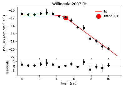
[[Fit Statistics]]
    # fitting method   = emcee
    # function evals   = 500000
    # data points      = 15
    # variables        = 3
    chi-square         = 10.7221275
    reduced chi-square = 0.89351063
    Akaike info crit   = 0.96389095
    Bayesian info crit = 3.08804156
[[Variables]]
    T:      5.05845001 +/- 0.16610447 (3.28%) (init = 5.052663)
    F:     -11.9760807 +/- 0.11941660 (1.00%) (init = -11.97601)
    alpha:  1.63903427 +/- 0.08893350 (5.43%) (init = 1.63728)
    t:      0 (fixed)

to_df(data_space='lin')

Function that returns a Pandas DataFrames of the lightcurve data.

You can specify the data to be returned in either logarithmic (log) or linear (lin) space.

Each DataFrame contains the following columns:

1. time_sec : The time of the datapoint in seconds (xdata)

2. flux : The flux of the datapoint in erg cm\(^{-2}\) s\(^{-1}\) (ydata)

3. flux_err : The flux error of the datapoint in erg cm\(^{-2}\) s\(^{-1}\) (yerr)

4. **attrsAny additional attributes of the datapoint as given in the

   instantiation of the Lightcurve object.

Parameters

data_space (str, {"log", "lin"}, optional) – Whether the data returned will be in logarithmic or linear space, by default “log”

Returns

data

Return type

pd.DataFrame

Raises

ValueError – If any “space” other than “log” and “lin” are specified.

to_dict(data_space='lin')

Function that returns a dictionary of the lightcurve data.

You can specify the data to be in either logarithmic (log) or linear (lin) space.

Each dictionary contains the following keys:

1. time_sec : The time of the datapoint in seconds (xdata)

2. flux : The flux of the datapoint in erg cm\(^{-2}\) s\(^{-1}\) (ydata)

#. flux_err : The flux error of the datapoint in erg cm\(^{-2}\) s\(^{-1}\) (yerr) #. **attrs : Any additional attributes of the datapoint as given in the instantiation of the Lightcurve object.

Parameters

data_space (str, {"log", "lin"}, optional) – Whether the data returned will be in logarithmic or linear space, by default “lin”

Returns

data

Return type

dict

Raises

ValueError – If any “space” other than “log” and “lin” are specified.

grblc.fitting.model module

class grblc.fitting.model.Model(func: Callable, name: str = '', slug: str = '', func_args: Optional[List[grblc.fitting.model.Parameter]] = None, bounds: Optional[list] = None)

Bases: object

Model class for use with the Lightcurve class.

This class is a wrapper around a function that can be used to fit a lightcurve.

Parameters

• func (Callable) – Function to fit to.

• name (str, optional) – Name to the function, by default the variable name of func

• slug (str, optional) – The shortened and simplified name of the function, by default name

• func_args (Dict[str, Parameter], optional) – Function arguments in the form of a list of Parameter, by default None

• bounds (list, optional) – Bounds by which x may be varied in fitting, by default [-np.inf, np.inf, -np.inf, np.inf]

Raises

ValueError – Makes sure all parameter names in func_args are actual parameters to the function.

classmethod SIMPLE_BPL()

Simple broken power law model

This is an empirical piece-wise model for GRB lightcurve afterglows.

The function is as follows:

\[\begin{split}f(t) = \left \{ \begin{array}{ll} \displaystyle{F_i \left (\frac{t}{T_i} \right)^{-\alpha_1} } & {\rm for} \ \ t < T_i \\ \displaystyle{F_i \left ( \frac{t}{T_i} \right )^{-\alpha_2} } & {\rm for} \ \ t \ge T_i, \\ \end{array} \right . \end{split}\]

where the transition from the exponential to the power law occurs at the point (\(T_i\), \(F_i\)), \(\alpha_1\) determines the temporal decay index of the initial power law, and \(\alpha_2\) is the temporal decay index of the final power law.

As implemented, log space is used for the time (sec) and flux (erg cm\(^{-2}\) s\(^{-1}\)). This means that for a light curve in which the afterglow plateau phase ends at 10,000 seconds corresponds to a \(T_i\) of 5.

Pre-defined priors on these parameters are:

• T : Uniform(1e-10, 10)

• F : Uniform(-20, 2)

• \(\alpha_1\) : Uniform(-5, 5)

• \(\alpha_2\) : Uniform(-5, 5)

Returns

The simple broken power law model.

Return type

Model

An example lightcurve is shown below:

import matplotlib.pyplot as plt
import numpy as np
import grblc
%matplotlib inline

sbpl = grblc.Model.SIMPLE_BPL()
x = np.linspace(2, 8, 100)
T, F, alpha1, alpha2 = p = 5, -12, -0.1, 1.5
y = sbpl(x, *p)
plt.plot(x, y)
plt.title(sbpl.name)
plt.xlabel("log Time (s)")
plt.ylabel("log Flux (erg cm$^{-2}$ s$^{-1}$)")
plt.show()

classmethod SMOOTH_BPL()

Smooth broken power law model

This is an empirical piece-wise model for GRB lightcurve afterglows.

The function is as follows:

\[f(t) = F_i \left (\left (\frac{t}{T_i} \right )^{S\alpha_1} + \left (\frac{t}{T_i} \right )^{S \alpha_2} \right )^{-\frac{1}{S}}\]

where the transition from the exponential to the power law occurs at the point (\(T_i\), \(F_i\)), \(\alpha_1\) determines the temporal decay index of the initial power law, and \(\alpha_2\) is the temporal decay index of the final power law, and \(S\) is the smoothing factor.

As implemented, log space is used for the time (sec) and flux (erg cm\(^{-2}\) s\(^{-1}\)). This means that for a light curve in which the afterglow plateau phase ends at 10,000 seconds corresponds to a \(T_i\) of 5.

Pre-defined priors on these parameters are::

• \(T_i\) : Uniform(1e-10, 10)

• \(F_i\) : Uniform(-20, 2)

• \(\alpha_1\) : Uniform(-5, 5)

• \(\alpha_2\) : Uniform(-5, 5)

• \(S\) : Uniform(-inf, inf)

Returns

The simple broken power law model.

Return type

Model

An example lightcurve is shown below:

import matplotlib.pyplot as plt
import numpy as np
import grblc
%matplotlib inline

sbpl = grblc.Model.SMOOTH_BPL()
x = np.linspace(2, 8, 100)
T, F, alpha1, alpha2, S = p = 5, -12, -0.1, 1.5, 0.5
y = sbpl(x, *p)
plt.plot(x, y)
plt.title(sbpl.name)
plt.xlabel("log Time (s)")
plt.ylabel("log Flux (erg cm$^{-2}$ s$^{-1}$)")
plt.show()

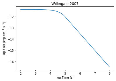
classmethod W07(vary_t=True)

Willingale et al. (2007) model

This is a phenomenological model for GRB lightcurve afterglows popularized in the paper by Willingale et. al, (2007). 1

Taken from his paper, it is as follows:

\[\begin{split}f(t) = \left \{ \begin{array}{ll}\displaystyle{F_i \exp{\left ( \alpha_i \left( 1 - \frac{t}{T_i} \right) \right )} \exp{\left (- \frac{t_i}{t} \right )}} & {\rm for} \ \ t < T_i \\ ~ & ~ \\ \displaystyle{F_i \left ( \frac{t}{T_i} \right )^{-\alpha_i} \exp{\left ( - \frac{t_i}{t} \right )}} & {\rm for} \ \ t \ge T_i, \\\end{array} \right .\end{split}\]

where the transition from the exponential to the power law occurs at the point (\(T_i\), \(F_i\)), \(\alpha\) determines the temporal decay index of the power law, and \(t_i\) is the time of the initial rise of the lightcurve.

As implemented, log space is used for the time (sec) and flux (erg cm\(^{-2}\) s\(^{-1}\)). This means that for a light curve in which the afterglow plateau phase ends at 10,000 seconds corresponds to a \(T_i\) of 5.

Pre-defined priors on these parameters are:

• \(T_i\) : Uniform(1e-10, 10)

• \(F_i\) : Uniform(-20, 2)

• \(\alpha\) : Uniform(0, 5)

• \(t\) : Uniform(0, inf)

Parameters

vary_t (bool, optional) – The fourth parameter to this Model, t, often does not vary the lightcurve in any way and thus is sometimes set to zero. This allows the user to make the fitter not vary it. Otherwise, you can set the vary parameter to zero via Model[Parameter.name].vary = False. By default True.

Returns

The Willingale et al. (2007) model.

Return type

Model

An example lightcurve is shown below:

import matplotlib.pyplot as plt
import numpy as np
import grblc
%matplotlib inline

w07 = grblc.Model.W07()
x = np.linspace(2, 8, 100)
T, F, alpha, t = 5, -12, 1.5, 1
y = w07(x, T, F, alpha, t)
plt.plot(x, y)
plt.title(w07.name)
plt.xlabel("log Time (s)")
plt.ylabel("log Flux (erg cm$^{-2}$ s$^{-1}$)")
plt.show()

1

https://arxiv.org/abs/astro-ph/0612031

property func: Callable

property func_args: Dict[str, grblc.fitting.model.Parameter]

class grblc.fitting.model.Parameter(name: str, description: Optional[str] = None, min: float = - inf, max: float = inf, vary: bool = True, plot_fmt: Optional[str] = None)

Bases: object

Parameter class for use with the Model class.

This class is used to store the information about a parameter in a model. Information includes the name, description, parameter priors, and whether the parameter is to be varied in fitting.

Parameters

• name (str) – Parameter name.

• description (str, optional) – Description of the parameter, by default None

• min (float, optional) – Minimum possible value of the parameter, by default -np.inf

• max (float, optional) – Maximum possible value of the parameter, by default np.inf

• vary (bool, optional) – Controls whether the variable will be allowed to vary in fitting, by default True

• plot_fmt (str, optional) – LaTeX form of the parameter name to be plotted, by default the same as name.

grblc.fitting.model.chisq(x, y, sigma, model, p, return_reduced=False)

A function to calculate the chi-squared value of a given proposed solution:

\[\chi^2 = \sum_{i=1}^N \frac{(y_i - f(x_i))^2}{\sigma_i^2}\]

The reduced \(\chi^2\) value, \(\chi^2_\nu\), can also be returned, and is calculated as:

\[\chi^2_\nu = \frac{\chi^2}{{\rm \# ~data~ points} - {\rm \# ~free~ params}}\]

Parameters

• x (array_like) – The x and y values of the data points.

• y (array_like) – The x and y values of the data points.

• sigma (array_like) – Standard error of the data points.

• model (callable) – The model to be fit to the data. Should take the form of a function that takes x, parameters p, and returns y in the form of y = model(x, *p).

• p (array_like) – List of parameter values to be used in the model.

• return_reduced (bool, optional) – Determines whether the reduced \(\chi^2\) will be returned as well, by default False

Returns

\(\chi^2\) for each point in the dataset, along with the reduced \(\chi^2\) value (if return_reduced=True)

Return type

numpy.ndarray

grblc.fitting.outlier module

class grblc.fitting.outlier.OutlierPlot(filename: Optional[str] = None, data=None, name: Optional[str] = None, plot=True, hover_labels: Optional[list] = None, legend_label: Optional[str] = None)

Bases: object

init_plot(hover: Optional[list] = None, legend_label: Optional[str] = None)

classmethod outlier_check_(data, save=False)

static prompt()

update(key, save=False)

update_plot()

Module contents